
Placing oblique photos on the map
/[This post also appears on the Mountain Legacy Project website. You can check out the MLP blog here.]
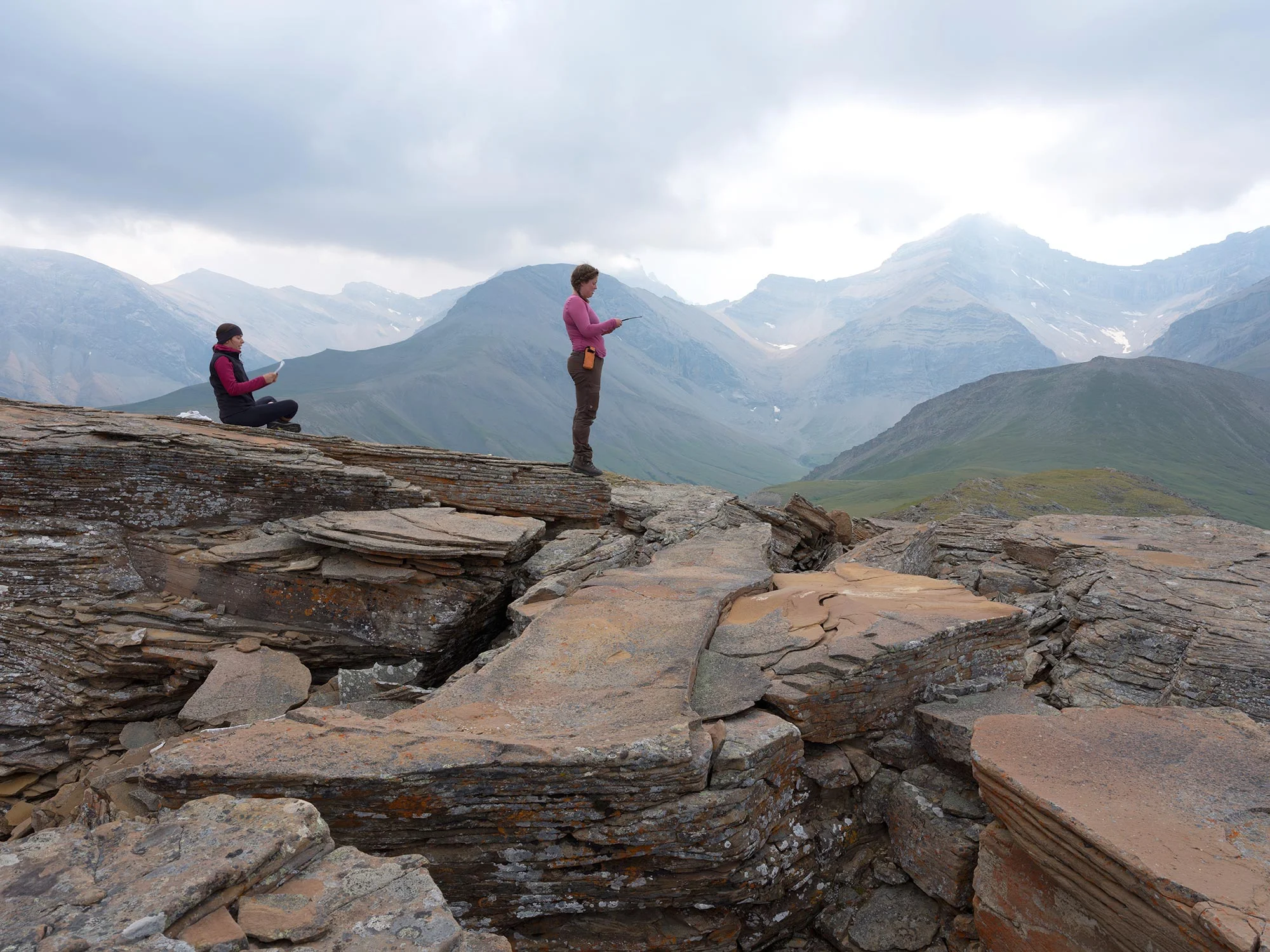
The Landscapes in Motion Oblique Photo Team has the daunting task of scaling mountains to repeat photographs taken up to a century ago by land surveyors. In previous posts we’ve described how these intrepid researchers locate sites, line up their photos, and what it’s like working in the field. With the summer fieldwork over, we now get to learn how they are harnessing technology to analyze landscapes in these repeat photographs and collect data from them.
We talk a lot about the Landscapes in Motion Oblique Photo Team, but what exactly does “oblique photo” mean?
Looking at the world from a different angle
Typically, people studying landscapes use images taken from satellites or airplanes. These “bird’s eye view” images are nice because they are almost perfectly perpendicular to the Earth’s surface—the kind of image you get when you switch to “Satellite View” on Google Maps. Each pixel corresponds to a fixed area (e.g. 30 m by 30 m) and represents a specific real-world location (e.g., a latitude and longitude).

Example of a satellite image. Landsat 8, path 42 row 25, August 22nd 2018. This image cuts through Calgary at the top and reaches south past Crowsnest Pass. Each pixel in this satellite image corresponds to a 30 m by 30 m square on the ground. Image courtesy USGS Earth Explorer.
The Oblique Photo Team, on the other hand, deals with historical and repeat photographs from the Mountain Legacy Project (MLP). These photos are taken from the ground, at an “oblique” angle—like switching to “Street View” on Google Maps. Pixels closer to the camera represent a smaller area than pixels farther away[i], and it is difficult to know the exact real-world location of each pixel on a map.
Difficult, but not impossible.

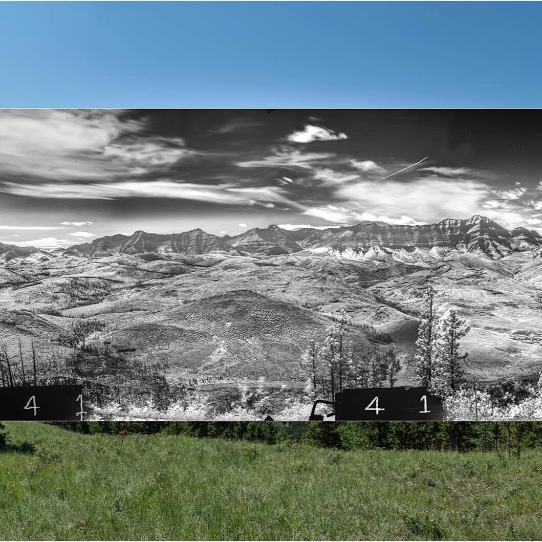
Example of an oblique image. This photograph of Crowsnest Mountain was taken in 1913 by surveyor Morrison Parsons Bridgland, from Sentry Mountain, and was repeated by the Mountain Legacy Project in 2006. Photo courtesy of the Mountain Legacy Project.
Given the incredible historical timeline captured by MLP photo pairs (the historical photos were captured over 100 years ago), it is worth overcoming this challenge. By comparing pairs of photos, we have the unique opportunity to see how vegetation cover types have changed (e.g., from evergreen forest to open meadow) over many decades. These differences are obvious when paired oblique photos are compared, but more challenging to quantify. Thus, we have taken on the difficult but not impossible challenge of developing a tool to assign real-world locations to each pixel of an oblique photograph.
While several similar tools already exist[i], most require heavy user input: for instance, someone has to sit at a computer and select corresponding points between oblique photos and 2D maps. Given the vastness of the MLP collection and the size of our study area, this could take years. So, we are building a way to automate the process, making it fast, scalable and accurate.
“How will you do this,” you ask? A little bit of elevation data, a little bit of camera information, a little bit of math and a whole lot of programming.
The Tool
The tool we are developing is a part of the MLP’s Image Analysis Toolkit. Let us run you through the steps we take to get to the final product: a 2D map as viewed from above!
Step 1: The Digital Elevation Map
We first need a Digital Elevation Model (DEM). A DEM is a map in which each pixel has a number that represents its elevation. We also need to know camera position (where it is:e.g., latitude, longitude, elevation) and orientation (where it is facing: e.g., azimuth, tilt and inclination), plus the camera’s field of view.

Example of a Digital Elevation Model. Darker colours indicate lower elevations and lighter colours indicate higher elevations. Image courtesy of Japan Aerospace Exploration Agency (©JAXA).
Step 2: The Virtual Image
Using the DEM we next create a “virtual image”: a silhouette of what can be seen from the specified camera location and orientation. To do so, we trace an imaginary line from each pixel in the DEM to the camera and see where it falls within the photo frame.

Example of a virtual image generated from a point atop Sentry Mountain, facing Crowsnest Mountain.
Step 3: The Virtual Photograph
Have you ever zoomed into the mountains on Google Earth and switched to “ground-level view”? When that happens, Google Earth basically shows satellite images from an oblique angle. It does this in places that are remote and don’t have Street View photos.
With our “virtual photograph” tool, we do more or less the same thing: we repeat the process of creating a virtual image, this time mapping satellite image pixels onto it. This step can be helpful for looking at areas where repeat photographs haven’t been taken.


Left: Example of ground-level view in the mountains in Google Earth. Right: Example of a virtual photograph generated from satellite imagery for Crowsnest Mountain. Satellite imagery courtesy of Alberta Agriculture and Forestry.
Step 4: The Viewshed
This brings us to the point where we have a photograph (say, a historical or repeat photograph), and we want to calculate the area of different landscape types in the photo (e.g., a forest or meadow). To do this, we need to know the real-world location of each pixel in the oblique photo.
We use math to map out where each oblique photo pixel belongs on the DEM. This is like the reverse of the “virtual image” from earlier. This creates a map, which we call a “viewshed”, showing the parts of the landscape that are actually visible within the photograph.

Example of a viewshed. Each blue pixel should be visible from the given camera location & orientation. Each white pixel cannot be seen in the oblique photo view. (Green pixels represent the foreground and black pixels are outside of the camera’s field of view). Photo courtesy of the Mountain Legacy Project.
Now we know where each pixel from an oblique photo gets mapped to on the DEM—so we know where each pixel of the photo exists on the ground! And, because we know that each pixel of the DEM is of a fixed size (e.g. 5 m by 5 m), we can estimate the area covered by oblique photo pixels.
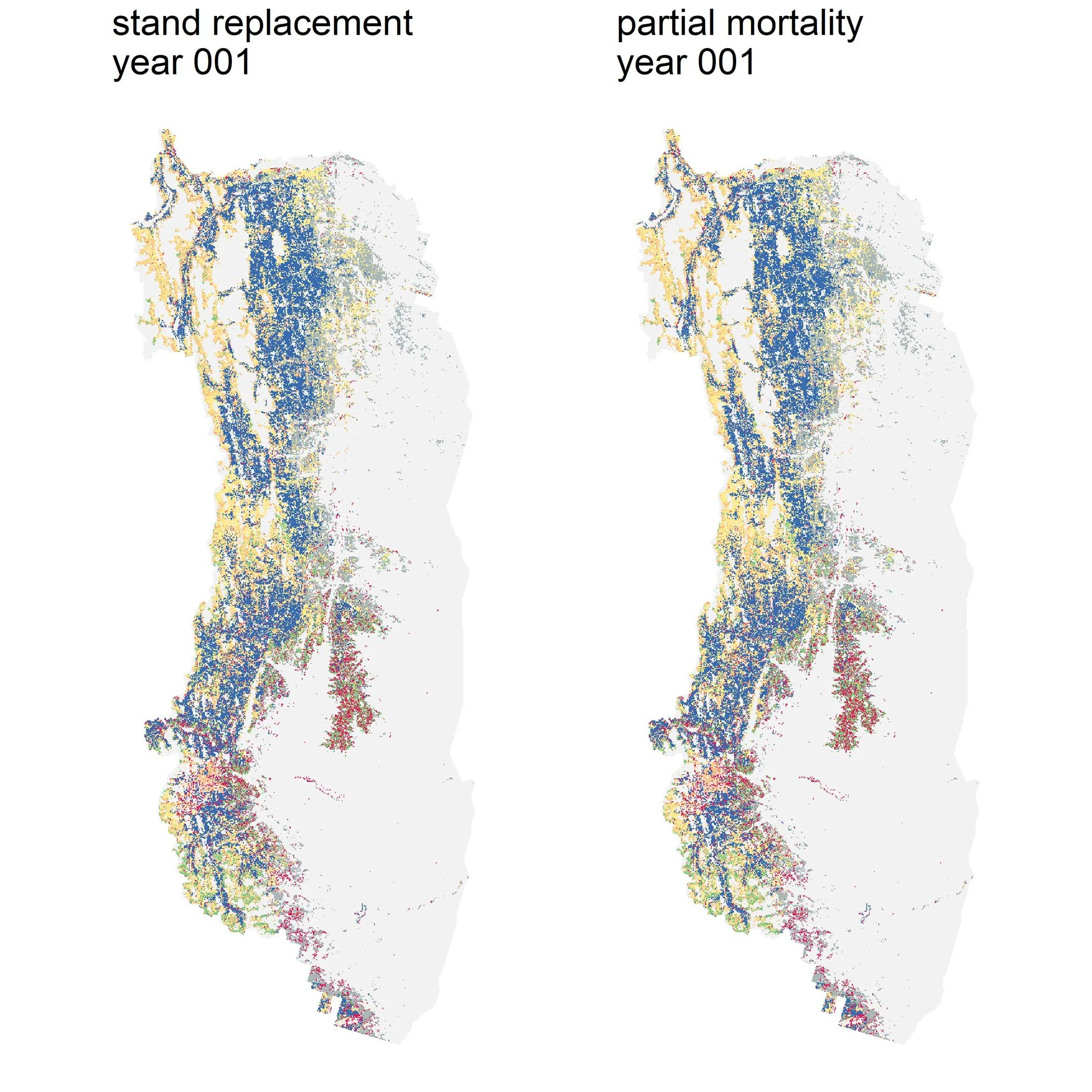
This process will allow us to take a historical or repeat photo and compute the true area covered by different forest types, meadows, burned forest, and more.
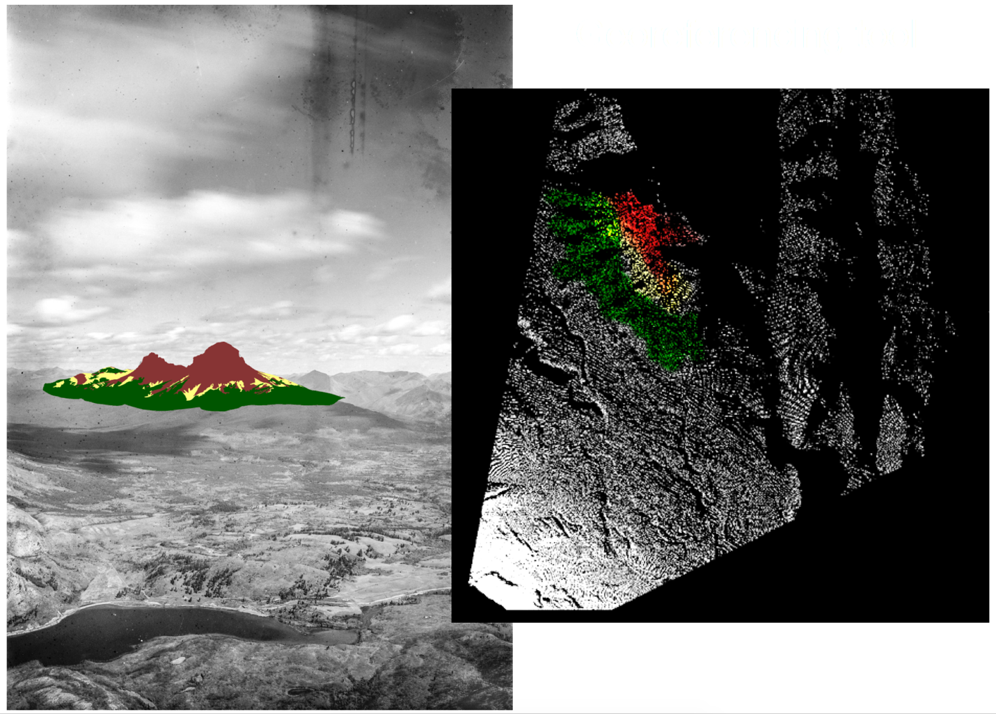
Left: the same historical photograph as above of Crowsnest Mountain, this time with different land cover types drawn onto it (rock in red, alpine meadow in yellow, forest in green). Right: the accompanying viewshed, showing where those coloured areas exist in 2D. In the viewshed image, we can count how many pixels are red, yellow or green, multiply those numbers by 25 (because each pixel measures 5 m by 5 m), and estimate the area covered by rock, alpine meadow or forest. Note: these visuals are using preliminary data and are for demonstration purposes only. Images by J. Fortin and M. Whitney.
Software advances to move Landscapes in Motion forward
The Oblique Photo Team is currently ironing out some kinks in the tool such as accounting for the curvature of the Earth. But soon, this tool will allow us to map out differences and similarities between historical and repeat photo pairs.
These comparisons will let us build timelines of landscape condition within the Landscapes in Motion study area—not only when things changed, but exactly where they changed and by how much. This information can then be used by Ceres Barros with the Modelling Team to build more complete models of landscape change. Ultimately, it becomes a piece of the puzzle that helps our research team better understand the mechanisms of change in the forested landscapes of southwestern Alberta.
Julie Fortin is a recent Master's graduate and research assistant with the Mountain Legacy Project, and a member of the Oblique Photography Team with Landscapes in Motion.
Michael Whitney is a research assistant and software developer working with the Mountain Legacy Project and Landscapes in Motion.
Every member of our team sees the world a little bit differently, which is one of the strengths of this project. Each blog posted to the Landscapes in Motion website represents the personal experiences, perspectives, and opinions of the author(s) and not of the team, project, or Healthy Landscapes Program.
[i] Imagine a photo taken with people (say, football players) in the foreground and a crowd in the background. Now divide this photo into a grid of squares—these will be like our “pixels”. A square on the person right up by the camera might cover just part of their face, while a square on the crowd at the back might capture several people! This is what it means for a pixel to represent a smaller area closer to the camera (e.g., a face), and a larger area farther from the camera (e.g., several people).
[i] See for example the WSL Monoplotting Tool, JUKE method, PCI Geomatica Orthoengine, Barista, Corripio, QGIS Pic2Map